Generalized Linear Models

Generalized Linear Models in Python

import numpy as np
from numpy.random import uniform, normal, poisson, binomial
from scipy import stats
import statsmodels.api as sm

import matplotlib.pyplot as plt
%matplotlib inline
import seaborn as sns
sns.set()

# Generate example data
np.random.seed(42)  # Set seed for reproducibility

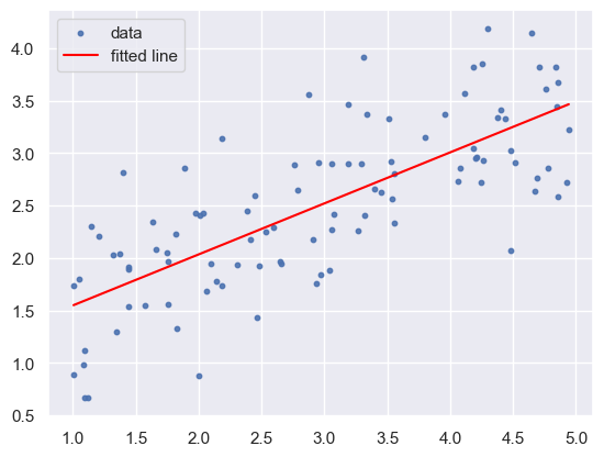
1. Linear Regression

# generate simulation data
np.random.seed(5)
n_sample = 100
a = 0.5
b = 1
sd = 0.5

x = uniform(1, 5, size=n_sample)
mu = a * x + b # linear predictor is a * x + b, link function is y=x
y = normal(mu, sd) # Probability distribution is normal distribution

slope, intercept, r_value, p_value, std_err  = stats.linregress(x, y)
xvals = np.array([min(x), max(x)])
yvals = slope * xvals + intercept
print(f'actual slope is {a}, estimated slope is {slope:0.4f}')
print(f'actual intercept is {b}, estimated intercept is {intercept:0.4f}')
print(f'actual standard error is {sd}, estimated standard error is {std_err:0.4f}')
print(f'p-value of the model is {p_value:0.4f}')

actual slope is 0.5, estimated slope is 0.4865
actual intercept is 1, estimated intercept is 1.0601
actual standard error is 0.5, estimated standard error is 0.0432
p-value of the model is 0.0000

plt.scatter(x, y, s=10, alpha=0.9, label='data')
plt.plot(xvals, yvals, color='red', label='fitted line')
plt.legend()

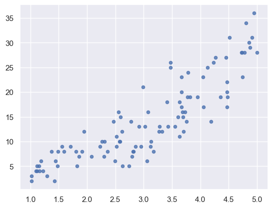
2. Poisson Regression

Three cases when Poisson Regression should be applied:
a. When there is an exponential relationship between x and y
b. When the increase in X leads to an increase in the variance of Y
c. When Y is a discrete variable and must be positive

# generate simulation data
n_sample = 100
a = 0.5
b = 1

x = uniform(1, 5, size=n_sample) 
mu = np.exp(a * x + b) # Linear predictor is a * x + b, 
                       # Link function is log function 
                       # (This is why x and y should have an exponential relationship)
y = poisson(mu) # Probability distribution is Poisson Distribution (This is why Y is a positive discrete variable)  
plt.scatter(x, y,  s=20, alpha=0.8)

exog, endog = sm.add_constant(x), y

# Poisson regression
mod = sm.GLM(endog, exog, family=sm.families.Poisson(link=sm.families.links.log()))
res = mod.fit()
display(res.summary())

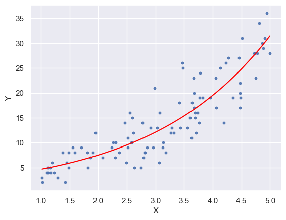
y_pred = res.predict(exog)

idx = x.argsort()
x_ord, y_pred_ord = x[idx], y_pred[idx]
plt.plot(x_ord, y_pred_ord, color='red')
plt.scatter(x, y,  s=10, alpha=0.9)
plt.xlabel("X")
plt.ylabel("Y")

/Users/steve.han/miniconda3/lib/python3.11/site-packages/statsmodels/genmod/families/links.py:13: FutureWarning: The log link alias is deprecated. Use Log instead. The log link alias will be removed after the 0.15.0 release.
  warnings.warn(

Generalized Linear Model Regression Results

Dep. Variable:	y	No. Observations:	100
Model:	GLM	Df Residuals:	98
Model Family:	Poisson	Df Model:	1
Link Function:	log	Scale:	1.0000
Method:	IRLS	Log-Likelihood:	-263.39
Date:	Sat, 06 Apr 2024	Deviance:	94.720
Time:	01:20:47	Pearson chi2:	95.3
No. Iterations:	4	Pseudo R-squ. (CS):	0.9775
Covariance Type:	nonrobust

	coef	std err	z	P>|z|	[0.025	0.975]
const	1.0606	0.096	10.996	0.000	0.872	1.250
x1	0.4778	0.026	18.627	0.000	0.428	0.528

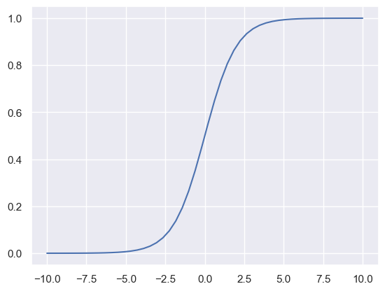
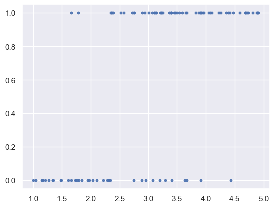
3. Logistic Regression

## logistic function
def logistic(x):
    return 1 / (1 + np.exp(-x))


xx = np.linspace(-10, 10)
plt.plot(xx, logistic(xx))

n_sample = 100
a = 1.5
b = -4

x = uniform(1, 5, size=n_sample)
x = np.sort(x)

q = logistic(a * x + b) # Linear predictor is a * x + b, 
                        # Link function is logit function 
y = binomial(n=1, p=q) # Probability distribution is binomial distribution (Bernoulli distribution can be other option)
plt.scatter(x, y,  s=10, alpha=0.9)

<matplotlib.collections.PathCollection at 0x138a3ca90>

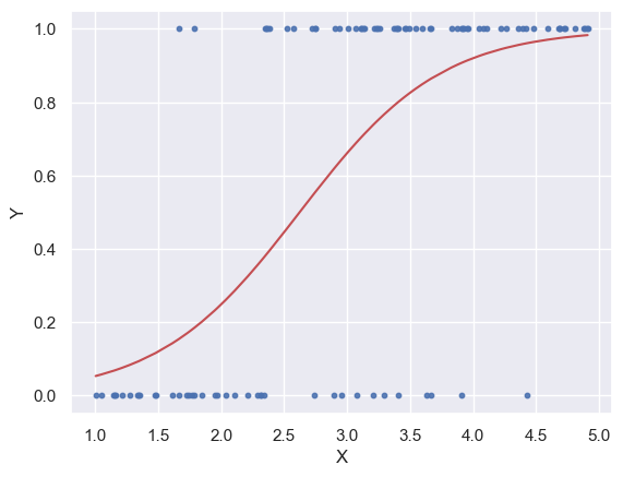
exog, endog = sm.add_constant(x), y

# Logistic regression
mod = sm.GLM(endog, exog, family=sm.families.Binomial(link=sm.families.links.logit()))
res = mod.fit()
display(res.summary())

y_pred = res.predict(exog)

idx = x.argsort()
x_ord, y_pred_ord = x[idx], y_pred[idx]
plt.plot(x_ord, y_pred_ord, color='r')
plt.scatter(x, y,  s=10, alpha=0.9)
plt.xlabel("X")
plt.ylabel("Y")

/Users/steve.han/miniconda3/lib/python3.11/site-packages/statsmodels/genmod/families/links.py:13: FutureWarning: The logit link alias is deprecated. Use Logit instead. The logit link alias will be removed after the 0.15.0 release.
  warnings.warn(

Generalized Linear Model Regression Results

Dep. Variable:	y	No. Observations:	100
Model:	GLM	Df Residuals:	98
Model Family:	Binomial	Df Model:	1
Link Function:	logit	Scale:	1.0000
Method:	IRLS	Log-Likelihood:	-42.196
Date:	Sat, 06 Apr 2024	Deviance:	84.392
Time:	01:32:33	Pearson chi2:	101.
No. Iterations:	5	Pseudo R-squ. (CS):	0.3896
Covariance Type:	nonrobust

	coef	std err	z	P>|z|	[0.025	0.975]
const	-4.6545	0.987	-4.714	0.000	-6.590	-2.719
x1	1.7746	0.340	5.214	0.000	1.108	2.442

Text(0, 0.5, 'Y')

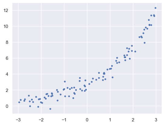
4. Custom GLM

Let’s create a glm model with conditions below
a. The relationship between x and y is an exponential relationship
b. The variance of y is constant when x increases
c. y can be either discret or continuous variable and also can be negative

# generate simulation data
n_sample = 100
a = 0.5
b = 1
sd = 0.5

x = uniform(-3, 3, size=n_sample) 
mu = np.exp(a * x + b) # Linear predictor is a * x + b, 
                       # Link function is log function 
                       # (This is why x and y should have an exponential relationship)
y = normal(mu, sd) # Probability distribution is Normal Distribution
plt.scatter(x, y,  s=10, alpha=0.9)

<matplotlib.collections.PathCollection at 0x138c3c610>

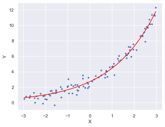
exog, endog = sm.add_constant(x), y

mod = sm.GLM(endog, exog, family=sm.families.Gaussian(link=sm.families.links.log()))
res = mod.fit()
display(res.summary())

y_pred = res.predict(exog)

idx = x.argsort()
x_ord, y_pred_ord = x[idx], y_pred[idx]
plt.plot(x_ord, y_pred_ord, color='red')
plt.scatter(x, y,  s=10, alpha=0.9)
plt.xlabel("X")
plt.ylabel("Y")

/Users/steve.han/miniconda3/lib/python3.11/site-packages/statsmodels/genmod/families/links.py:13: FutureWarning: The log link alias is deprecated. Use Log instead. The log link alias will be removed after the 0.15.0 release.
  warnings.warn(

Generalized Linear Model Regression Results

Dep. Variable:	y	No. Observations:	100
Model:	GLM	Df Residuals:	98
Model Family:	Gaussian	Df Model:	1
Link Function:	log	Scale:	0.27094
Method:	IRLS	Log-Likelihood:	-75.601
Date:	Sat, 06 Apr 2024	Deviance:	26.552
Time:	01:44:12	Pearson chi2:	26.6
No. Iterations:	6	Pseudo R-squ. (CS):	1.000
Covariance Type:	nonrobust

	coef	std err	z	P>|z|	[0.025	0.975]
const	0.9964	0.025	40.561	0.000	0.948	1.045
x1	0.4940	0.011	46.129	0.000	0.473	0.515

Text(0, 0.5, 'Y')